Instrumental variables estimation
What If: Chapter 16
Elena Dudukina
2022-03-21
1 / 17
16.1 The three instrumental conditions
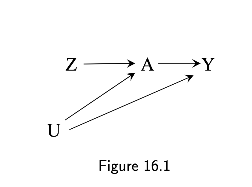
- RCT
- Z is the randomization assignment
- A is an indicator for receiving treatment
- Y is the outcome
- U is all factors (some unmeasured) that affect both the outcome and the adherence to the assigned treatment A
- Need to ensure conditional exchangeability of the treated and the untreated
- Closing backdoor A ⬅ U ➡ Y not feasible when U or its components are unmeasured
- Alternatively, can use non-backdoor approach
- Z is an instrumental variable (IV)
- Z is a causal instrument
2 / 17
16.1 The three instrumental conditions
- Z is associated with A
- Z does not affect Y except through its potential effect on A
- Z and A do not share causes
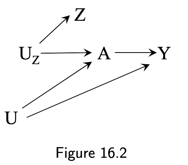
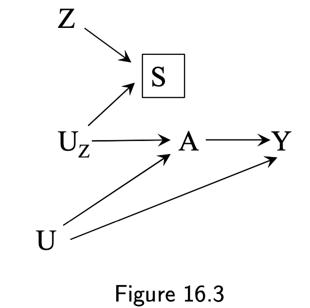
- \(U_z\) is a proxy instrument
- 16.2 \(U_z\) is a common cause of A and Z
- 16.3 \(U_z\) are associated due to conditioning on S
3 / 17
16.1 The three instrumental conditions
- Z: the price of cigarettes
- Check that Z and A are associated
- \(Pr[A = 1|Z = 1] − Pr[A = 1|Z = 0] > 0\)
data %>% group_by(highprice) %>% count(qsmk) %>% mutate( pct = n/sum(n) * 100 ) %>% filter(qsmk == 1, !is.na(highprice))## # A tibble: 2 × 4## # Groups: highprice [2]## highprice qsmk n pct## <dbl> <fct> <int> <dbl>## 1 0 1 8 19.5## 2 1 1 370 25.84 / 17
16.1 The three instrumental conditions
- Z is a weak instrument
- Conditions 2 and 3 cannot be empirically verified
5 / 17
16.2 The usual IV estimand
- The average causal effect of A on Y on the additive scale \(E[Y^{a=1}] - E[Y^{a=0}]\) is
- \(\frac{E[Y|Z=1]-E[Y|Z=0]}{E[A|Z=1]-E[A|Z=0]}\)
- numerator of the IV estimand is the average causal effect of Z on Y: intention-to-treat effect
- denominator is the average causal effect of Z on A: a measure of adherence to the assigned treatment A
- the higher the noncompliance, the bigger the difference between the effect of Z on Y and the effect of A on Y
6 / 17
16.2 The usual IV estimand
- IV estimand bypasses the need to adjust for the confounders
- numerator model: \(E[A|Z] = \alpha_0 +\alpha_1Z\)
- denominator model: \(E[Y|Z] = \beta_0 +\beta_1Z\)
# an instrument as weak if the F-statistic from the first-stage model is less than 10# two-stage-least-squares regressionlibrary(ivreg)ivreg(wt82_71 ~ qsmk | highprice, data = data) %>% broom::tidy(., conf.int = T) %>% filter(term == "qsmk1")## # A tibble: 1 × 7## term estimate std.error statistic p.value conf.low conf.high## <chr> <dbl> <dbl> <dbl> <dbl> <dbl> <dbl>## 1 qsmk1 2.40 19.8 0.121 0.904 -36.5 41.3# Chapter answer: 2.4 kg (-36.5; 41.3)7 / 17
16.2 The usual IV estimand
- Strong parametric assumptions for two-stage-least-squares regression
- Only valid as an estimator when the IV estimand can be interpreted as the average causal effect of treatment, whoch requires and additional assumption
8 / 17
16.3 A fourth identifying condition: homogeneity
- Homogeneity
- Constant effect of treatment A on outcome Y across all individuals (unrealistic)
- Smoking cessation made everyone in the study population gain (or lose) the same weight
- Equality of the average causal effect of A on Y across levels of Z in both the treated and in the untreated
- confounders U are not additive effect modifiers (unrealistic)
- Z-A association is constant across levels of the confounders U
- Can IV methods validly estimate the average causal effect of treatment without homogeneity assumption?
9 / 17
16.4 An alternative fourth condition: monotonicity
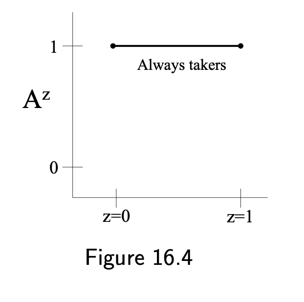
- Always-takers: \(A^{z=1}=1\) and \(A^{z=0}=1\)
- Never-takers: \(A^{z=1}=0\) and \(A^{z=0}=0\)
- Compliers: \(A^{z=1}=1\) and \(A^{z=0}=0\)
- Defiers: \(A^{z=1}=0\) and \(A^{z=0}=1\)
- "Monotonicity is not always a reasonable assumption in observational studies"
- No always-takers or defiers in RCTs by design
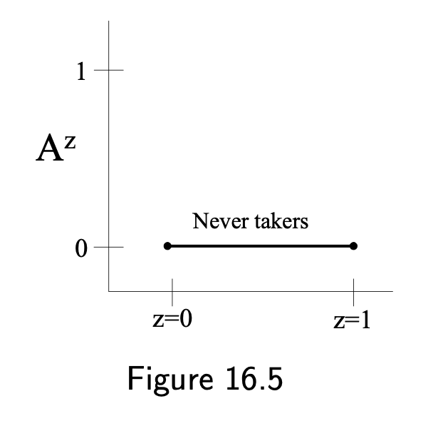
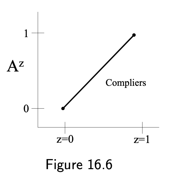
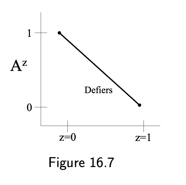
10 / 17
16.5 The three instrumental conditions revisited
- "Even in large samples, weak instruments introduce bias in the standard IV estimator and result in underestimation of its variance"
- "The effect estimate is in the wrong place and the width of the confidence interval around it is too narrow"
data %<>% mutate(highprice2 = if_else(price82 >= 1.6, 1, 0), highprice3 = if_else(price82 >= 1.7, 1, 0), highprice4 = if_else(price82 >= 1.8, 1, 0), highprice5 = if_else(price82 >= 1.9, 1, 0) )ivreg(wt82_71 ~ qsmk | highprice2, data = data) %>% broom::tidy(., conf.int = T) %>% filter(term == "qsmk1")## # A tibble: 1 × 7## term estimate std.error statistic p.value conf.low conf.high## <chr> <dbl> <dbl> <dbl> <dbl> <dbl> <dbl>## 1 qsmk1 41.3 165. 0.250 0.802 -282. 365.ivreg(wt82_71 ~ qsmk | highprice3, data = data) %>% broom::tidy(., conf.int = T) %>% filter(term == "qsmk1")## # A tibble: 1 × 7## term estimate std.error statistic p.value conf.low conf.high## <chr> <dbl> <dbl> <dbl> <dbl> <dbl> <dbl>## 1 qsmk1 -40.9 188. -0.218 0.828 -409. 327.ivreg(wt82_71 ~ qsmk | highprice4, data = data) %>% broom::tidy(., conf.int = T) %>% filter(term == "qsmk1")## # A tibble: 1 × 7## term estimate std.error statistic p.value conf.low conf.high## <chr> <dbl> <dbl> <dbl> <dbl> <dbl> <dbl>## 1 qsmk1 -21.1 28.4 -0.742 0.458 -76.9 34.7ivreg(wt82_71 ~ qsmk | highprice5, data = data) %>% broom::tidy(., conf.int = T) %>% filter(term == "qsmk1")## # A tibble: 1 × 7## term estimate std.error statistic p.value conf.low conf.high## <chr> <dbl> <dbl> <dbl> <dbl> <dbl> <dbl>## 1 qsmk1 -12.8 23.7 -0.541 0.588 -59.2 33.611 / 17
16.5 The three instrumental conditions revisited
- For each of additional definitions of a high price, the 95% confidence interval around the estimate is very wide but is an underestimate of the true uncertainty
- Stronger instrument that violates conditions 2 and 3 may be preferable to a more valid (less invalid) but weaker instrument
12 / 17
16.5 The three instrumental conditions revisited
- Condition 2 is unverifiable from the data
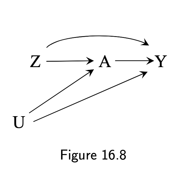
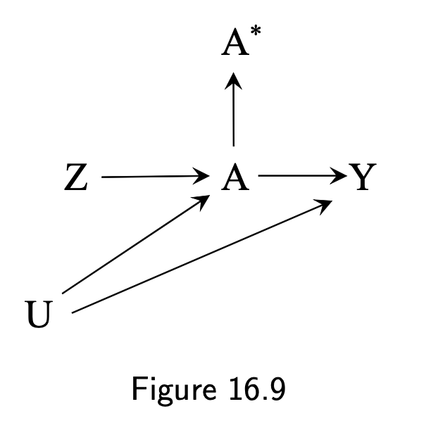
- Absence of a direct effect of the instrument on the outcome (violation on fig 16.8)
- May be violated when a continuous or multilevel treatment is dichotomized
- "Even if condition 2 holds for the original treatment A, it does not have to hold for its dichotomized version A∗, because the path Z → A → Y represents a direct effect of the instrument Z that is not mediated through the treatment A∗ whose effect is being estimated in the IV analysis (16.9)
13 / 17
16.5 The three instrumental conditions revisited
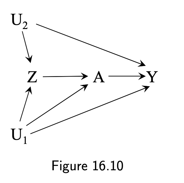
- Condition 3: confounding for the effect of the instrument on the outcome
- Unverifiable
- Adjust for known covariables
- Unverifiable assumption that there is no unmeasured confounding for the effect of Z on A within levels of the measured pre-instrument covariates V
- "Apply IV estimation repeatedly in each stratum of V, and pool the IV effect estimates under the assumption that the effect in the population (under homogeneity) or in the compliers (under monotonicity) is constant within levels of V"
14 / 17
16.5 The three instrumental conditions revisited
ivreg(wt82_71 ~ qsmk + sex + race + age + smokeintensity + smokeyrs + exercise + active + wt71 | highprice5 + sex + race + age + smokeintensity + smokeyrs + exercise + active + wt71, data = data) %>% broom::tidy(., conf.int = T) %>% filter(term == "qsmk1")## # A tibble: 1 × 7## term estimate std.error statistic p.value conf.low conf.high## <chr> <dbl> <dbl> <dbl> <dbl> <dbl> <dbl>## 1 qsmk1 -2.38 17.3 -0.138 0.891 -36.2 31.515 / 17
16.6 Instrumental variable estimation versus other methods
- IV estimation requires modeling assumptions even if infinite data (on super-popultion) were available
- Homogeneity condition is equal to setting to 0 the parameter corresponding to a product term in a structural mean model
- Estimation cannot be nonparametric
- Relatively minor violations of IV conditions "may result in large biases of unpredictable or counterintuitive direction"
- IV estimate may be more biased than an unadjusted estimate when IV conditions are violated
- Hard to think about common causes of IV and the treatment
- "Standard IV estimation is more restrictive than that for other methods" and "used to answer relatively simple causal questions"
16 / 17
References
- Hernán MA, Robins JM (2020). Causal Inference: What If. Boca Raton: Chapman & Hall/CRC (v. 30mar21)
- R ivreg package
17 / 17